A companion to silicon power usage, which walks the whole nine-step workflow from architectural budget to silicon measurement. This article goes deep on one question inside it: how do you get a power number from RTL, and how much should you believe it?
Every power estimate is wrong. The useful question is not whether — it is by how much, in which direction, and whether that is small enough to decide on. That question has an answer, it is quantifiable per method, and it is almost never stated in the tool documentation.
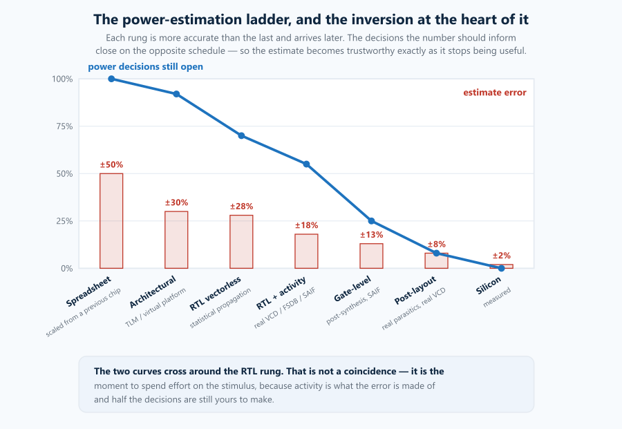
There is also an inversion at the heart of this that shapes everything else. The estimate gets more accurate as the design gets more concrete. The decisions the estimate should inform close on exactly the opposite schedule. By the time you can trust the number to 5%, there is almost nothing left you can do about it.
1. The two terms, and which one the method affects
Briefly, because the workflow article covers this properly.
Of the four factors in the dynamic term, an estimation method can measure well or badly, and and are given. — the activity factor — is the one that cannot be read off the design at all. It depends entirely on what the chip is doing, which means it depends on stimulus, which means it depends on a judgement about what the workload is.
That is why the accuracy of every rung below is dominated by the same thing, and why the tool you choose matters far less than most people assume.
Leakage behaves differently and more simply: it is a function of the standard cells present, their threshold flavours, the temperature and the voltage. Once a netlist exists, leakage estimates are good. Before one exists, they are a scaling argument.
2. The ladder
Seven rungs. For each: what it needs, what it can see, what it is structurally blind to, the tools, and the realistic error against final silicon.
On those error figures. They are typical industry numbers for a digital block in a mature flow, not measurements of any one design, and your own will differ — a team that has correlated two generations does considerably better than these, and a team using an unrepresentative workload does considerably worse. Treat them as the right order and the right ordering; the absolute value for your flow is something only correlation against your own silicon establishes, which is the argument section 2 closes on. Quoting ±18% as though it were a specification is exactly the mistake this article is written against.
Rung 0 — Spreadsheet, scaled from a previous design
Needs. A previous chip and a block diagram. Error: ±50% or worse.
Scale a known design by area, by node, by frequency, by gate count. It sounds unserious and it is not: at the moment it is used, nothing else exists, and it is the number that sizes the package, the regulator and the thermal solution. Those are long-lead decisions.
Blind to everything about this design that differs from the last one — which, if the architecture changed, is the answer.
The discipline that makes it worth anything: write down the assumptions as an explicit list, and revisit it at each later rung to see which one broke. A spreadsheet estimate with a documented assumption list is engineering; the same number without one is a guess wearing a suit.
Rung 1 — Architectural, from a virtual platform
Needs. A SystemC/TLM model, and power numbers per operation. Error: ±30%.
The model executes real software, counts operations — cache accesses, DMA transfers, DSP invocations, memory traffic — and multiplies by an energy-per-operation figure. The absolute number is mediocre; the relative comparison between two architectures is far better than that, because the errors are largely common-mode.
Tools. Synopsys Platform Architect, Cadence’s system design and verification flow, and a good deal of in-house spreadsheet-and-Python glue, which is honest.
Blind to implementation. It cannot know what synthesis will do, and it has no clock tree, no wires and no glitches.
Why it matters more than its error bar suggests: this is the rung with the most leverage. Choosing an accelerator over a software loop, halving memory traffic, or adding a cache level moves power by a factor. No downstream rung has decisions of that size available.
Rung 2 — RTL vectorless
Needs. RTL, a library, and a few assumed input toggle rates. Error: ±28%.
Statistical propagation: assume primary inputs toggle at some rate, propagate probabilities and toggle rates through the logic, get a per-node activity without simulating anything.
Tools. Ansys PowerArtist, Cadence Joules, Synopsys PrimePower in its RTL mode.
Blind to correlation and to reality. It does not know your bus is idle 90% of the time, that two blocks never run together, or that a FIFO is usually empty. Statistical propagation also systematically mishandles reconvergent fanout, because it treats correlated signals as independent.
When to use it. When RTL exists and representative stimulus does not — early in a project, or on a block whose testbench is not written. Treat it as a relative tool: it is good at ranking blocks by power and finding the ones worth attention, and poor at absolute numbers.
Rung 3 — RTL with real activity
Needs. RTL, a library, and a simulation of something representative. Error: ±18%.
The standard working rung. Simulate a real workload, dump the activity, feed it to the power tool.
Three activity formats, and choosing among them is a real decision:
| Format | What it holds | Size | Use it for |
|---|---|---|---|
| VCD | every transition, every net, timestamped | enormous | short windows, peak power, glitch analysis |
| FSDB | the same, compressed | large | the practical default when you need waveforms |
| SAIF | toggle counts and duty cycles, aggregated | small | average power over a long run |
The rule: average power needs SAIF; peak power and droop need waveforms. SAIF has thrown away the time axis, so it cannot tell you when the peak was.
Tools. PowerArtist, Joules, PrimePower.
Blind to the clock tree (it does not exist yet — the tool estimates it, and it is a large fraction of total power), to glitches below its modelling threshold, and to real wire capacitance.
What it is good for, and this is the important part: RTL power analysis tools do not just report a number. They report where the power is going and, increasingly, suggest specific RTL changes — clock-gating opportunities the synthesis tool will not find, registers that toggle when their output is unused, memory accesses that could be avoided. That diagnostic output is worth more than the total, because the total will be recomputed later anyway and the fix has to happen now.
Rung 4 — Gate-level, post-synthesis
Needs. A netlist, and activity mapped onto it. Error: ±13%.
Now the cells are real and their input capacitances come from the library rather than from an estimate. Wire capacitance is still a wire-load model or a virtual-route estimate.
Tools. PrimePower, Joules, PowerArtist.
Blind to real routing. The clock tree is now at least partly built, which removes one of the larger RTL uncertainties.
The trap: activity must be mapped from RTL names onto netlist names, and synthesis has renamed, merged, replicated and optimised away signals. A poor mapping silently reduces apparent activity and makes power look better. Check the mapping-rate report; anything below about 90% mapped is a number to distrust.
Rung 5 — Post-layout, with extracted parasitics
Needs. A routed design, SPEF, and real activity. Error: ±8%.
Every capacitance is extracted. The clock tree is real. This is the number that goes on the datasheet, and it is also the input to IR-drop and electromigration signoff and to dynamic voltage-drop analysis.
Tools. PrimePower with SPEF, Ansys RedHawk-SC and Cadence Voltus for the IR/EM side, Ansys Totem for analog.
Blind to very little in the model — but the residual ±8% is mostly still activity, plus library characterisation accuracy and the gap between the corner you analysed and the silicon you received.
Rung 6 — Silicon
Error: ±2%, which is the measurement itself.
And this is the rung that makes all the others honest. Measure a real part running a real workload, then go back and correlate: what did the post-layout model say for the same workload? The delta is your flow’s systematic error, and you now know its sign.
Nobody who has not done this knows whether their flow runs optimistic or pessimistic. A team that has correlated two generations can predict the third to within a few per cent, using exactly the same tools that gave someone else ±20%. The accuracy is in the calibration, not the licence.
3. Where the ±18% actually comes from
“Plus or minus twenty per cent” is only actionable if you know which term dominates. At the RTL-with-activity rung, for a typical digital block:
| Term | Contribution | Why |
|---|---|---|
| Activity () | ±12% | the stimulus is a proxy for a workload nobody has run yet |
| Capacitance | ±8% | wire-load model rather than extraction |
| Clock tree | ±7% | does not exist; estimated from fanout and an assumed topology |
| Glitch power | ±6% | spurious transitions RTL cannot represent |
| Library / corner | ±5% | voltage, temperature, process point vs the silicon you get |
Independent contributions combine in quadrature:
Two things follow, and they are the practical content of this article.
Halving the largest term beats eliminating the smallest. Take activity from ±12% to ±6% by investing in better stimulus and the total falls to ±14.5%. Eliminate the library term entirely — perfect characterisation, exactly the right corner, zero error — and the total falls only to ±17.1%. One of those is worth a week; the other is not worth an afternoon.
That is quadrature doing what quadrature does: once a term is well below the largest one, it has almost stopped contributing. Chasing the small terms is the most common way to spend effort on power accuracy and get nothing back.
A better tool does not move the dominant term. PowerArtist, Joules and PrimePower will give you answers within a few per cent of each other on the same design with the same activity. The choice between them is about diagnostics, capacity, runtime and what your flow already uses — not about accuracy. The accuracy is in the stimulus.
The term people forget: glitch power
A combinational node can transition several times before settling, because its inputs arrive at different times. Those transitions charge and discharge real capacitance and dissipate real power, and they do no useful work.
On arithmetic-heavy logic — multipliers, CRC trees, wide adders — glitch power is commonly 10–20% of dynamic power, and on a badly balanced design it can exceed 30%. RTL simulation is zero-delay or unit-delay, so it cannot see glitches at all: RTL power analysis estimates them statistically. This is one of the reasons an RTL estimate can be optimistic in a specific, structural way, and one of the reasons a gate-level number with real delays sometimes comes in above the RTL one rather than below.
4. The stimulus problem, which is the whole problem
If activity dominates the error, then the question “which power tool” is less important than “which ten microseconds of simulation”.
What does “representative” mean? It is not one thing, and asking for a single number is usually the mistake:
| You want | Run this | Report |
|---|---|---|
| Battery life, thermal budget | a long, realistic mixed workload | average over the whole run |
| Package and heatsink | the worst sustained mode | average over a thermal time constant |
| PDN and decoupling design | the worst burst | peak over a few clock cycles |
| Dynamic voltage drop | the worst simultaneous switching | instantaneous, per cycle |
| Thermal hotspot | the worst sustained mode, per block | average, spatially resolved |
These are different numbers from different windows, and a project that asks for “the power number” gets one of them and uses it for all five. The thermal answer averaged over a second is useless for dynamic voltage drop, which cares about a single cycle.
How to find the worst window. Run a long simulation with cheap per-cycle activity tracking, plot power against time, and then take the expensive detailed analysis only on the worst windows it identifies. Every modern tool supports this two-pass flow, and it is the difference between analysing 10 µs of simulation and 10 ms.
Beware the benchmark that is not your workload. Dhrystone and CoreMark exercise a CPU in a way nothing else does: tight loops, a working set small enough to stay in cache, almost no traffic reaching DRAM, and no accelerator activity at all. They are not memory-free — CoreMark does list processing and matrix work — but the memory they touch is the cheap kind, and DRAM is often the largest power term in the real system. A power number from a synthetic benchmark is a number about the benchmark.
Beware also the idle case. Many products spend most of their life mostly idle, and for those the number that decides battery life is leakage plus clock-tree power in a mostly-quiet state — which is a different simulation, and one nobody remembers to run.
5. What you can still do at each rung
This is the half that gets left out: the estimate exists to drive a decision, so what matters is which decisions are still open when it arrives.
| Rung | Still open | What the number should trigger |
|---|---|---|
| Spreadsheet | everything | package, regulator, thermal solution, product feasibility |
| Architectural | architecture, partitioning, memory hierarchy, accelerators | the big structural changes — nothing later is as effective |
| RTL vectorless | RTL structure, clock-gating strategy, power domains | rank blocks, target the worst; set the UPF architecture |
| RTL + activity | RTL changes, gating, operand isolation, memory access patterns | act on the tool’s diagnostics; this is the last cheap rung |
| Gate-level | synthesis strategy, Vt mix, a limited amount of RTL | re-target synthesis; multi-Vt; a little restructuring |
| Post-layout | placement, power grid, decap, a late ECO | fix IR/EM violations; add decap; not much else |
| Silicon | firmware, DVFS policy, binning | software power management — and the next chip |
Read the right-hand column downward and the shape of the problem is obvious. By the RTL rung you have spent most of your leverage and gained only half your accuracy. That crossing point is why the effort belongs there: it is the last place where a ±18% number can still change a decision that matters.
6. A worked example
A block estimated at RTL, then measured. The numbers are illustrative but the shape is what happens in practice.
| Stage | Estimate | Note |
|---|---|---|
| RTL + activity, first pass | 118 mW | synthetic benchmark stimulus |
| RTL + activity, real workload | 154 mW | +31% — the benchmark was not the workload |
| Gate-level, post-synthesis | 171 mW | +11% — clock tree now real, glitches now visible |
| Post-layout, extracted | 182 mW | +6% — real wire capacitance |
| Silicon, same workload | 176 mW | −3% against post-layout |
Two observations. The single biggest jump was changing the stimulus, not changing the tool — and it happened at the same rung, with the same software. And every step after the stimulus fix was an increase, which is the usual direction: RTL estimates tend to run optimistic because the things RTL cannot see — clock tree, glitches, real wires — all add power rather than remove it.
If your flow has never come in high, you have not correlated it.
7. Best practices
- Report a number with its method and its window. “182 mW” is not a result. “182 mW average, post-layout, extracted parasitics, workload X over 4 ms, 0.8 V, 85 °C, typical corner” is.
- Spend on the stimulus before the tool. It is the dominant error term at every rung where you can still act.
- Run more than one window — average, worst sustained, worst burst — and label them.
- Use vectorless as a ranking tool, never as an absolute one.
- Check the activity mapping rate at gate level. Below ~90% mapped, distrust the number.
- Correlate against silicon, and carry the correction forward. This is the single highest return on effort in the whole list, and almost nobody does it.
- Track the estimate over time as one chart. A number that has moved 40% since the last review is telling you something about your assumptions, not about your design.
- Budget the margin explicitly. If the estimate is ±18% and the thermal limit is 200 mW, an estimate of 180 mW is not passing — it is a coin flip.
8. The pitfalls
- Quoting a power number without its method, corner and window.
- Using a synthetic benchmark and calling it representative.
- Averaging away the peak, then being surprised by dynamic voltage drop.
- Buying a more accurate tool to fix an error that is made of stimulus.
- Trusting a gate-level number with a 60% activity mapping rate.
- Treating a vectorless absolute number as a budget.
- Forgetting the idle case on a product that is mostly idle.
- Comparing this quarter’s estimate to last quarter’s without checking that the workload, corner and method were the same.
- Never correlating against silicon, and therefore never learning the sign of your own error.
Glossary
Activity factor (α) — The fraction of clock cycles on which a node toggles, and the only term in that cannot be derived from the design. It comes from stimulus, which makes it a judgement about the workload rather than a measurement of the circuit, and it is the largest error term at every rung where you can still act on the answer.
Clock-gating efficiency — The fraction of register toggles actually suppressed by enable logic. A standard RTL power-tool diagnostic, and usually the first place a real saving is found, because synthesis only inserts the gating it can prove safe from the code as written.
Correlation — Comparing a model’s prediction against a measurement of real silicon running the same workload, and carrying the resulting correction forward. The difference between a flow with ±20% error and the same flow with ±8%, using identical tools.
Dynamic voltage drop (DvD) — Instantaneous supply droop from switching, as opposed to static IR drop. It needs per-cycle activity — an average has thrown away exactly the information it depends on.
FSDB — A compressed waveform database. The practical default when you need per-transition detail over a window long enough to be interesting.
Glitch power — Power burned by spurious transitions on combinational nodes whose inputs arrive at different times. Commonly 10–20% of dynamic power on arithmetic logic, invisible to zero-delay RTL simulation, and one structural reason RTL estimates run optimistic.
Mapping rate — The fraction of RTL activity successfully associated with netlist nodes after synthesis renamed, merged and optimised them. A low rate silently reduces apparent activity, so it makes power look better rather than worse — which is why it has to be checked rather than assumed.
Peak vs average power — Different questions with different answers from different windows. Average sets battery life and thermal; peak over a few cycles sets the PDN and the decoupling. Reporting one as the other is the most common power-number error.
SAIF — Switching Activity Interchange Format: aggregated toggle counts and duty cycles, without a time axis. Small and sufficient for average power; useless for peak, because the information about when has been discarded.
Vectorless estimation — Propagating assumed input toggle rates statistically rather than simulating. Useful before a testbench exists and for ranking blocks; poor in absolute terms, because it cannot know that your bus is idle most of the time and it treats reconvergent signals as independent.
VCD — Value Change Dump: every transition on every net, timestamped, in plain text. Complete, enormous, and the right input when you are hunting a peak or analysing glitches.
Wire-load model — A statistical estimate of wire capacitance from fanout, used before routing exists. The reason pre-layout capacitance carries an error bar at all, and superseded by extracted parasitics once there is a route.
Related reading
- Silicon power usage: the workflow — the nine-step flow this article zooms into, including UPF, power gating and the techniques worth their cost
- Power integrity, from IR drop to di/dt — what the peak number is for, on the board and on the die
- On-die signal integrity — extraction, corners and the parasitics that make the post-layout rung accurate
- The ASIC design flow — where each rung sits in the schedule
Further reading
Book links below are Amazon affiliate links: if you buy through one we earn a small commission at no extra cost to you. It does not influence what is recommended — the same books were on this list before the links were.
- Jan Rabaey, Low Power Design Essentials — the standard text, and strong on where the power physically goes.
- Michael Keating et al., Low Power Methodology Manual — methodology rather than physics; the practical companion to a real flow.
- Jan Rabaey, Anantha Chandrakasan and Borivoje Nikolić, Digital Integrated Circuits — the device-level grounding under all of it.
- Neil Weste and David Harris, CMOS VLSI Design — good on glitch power and on why balanced logic depth matters.
- IEEE 1801 (UPF) — the standard itself, for when the question is what is legal rather than what is fast.
Have a power number nobody trusts, or a thermal budget that depends on which window you averaged? That’s what we do. Reach us at circuit-design.space.
circuit-design.space · +1-971-357-1400 · anovickis@circuit-design.space