A companion to the signal-integrity series. Those posts use S-parameters constantly; this one explains what they actually are. The Smith chart guide covers the other half — how to read reflection graphically.
Every channel model, every connector datasheet, every VNA measurement and every field-solver result arrives as S-parameters, usually in a Touchstone file. They are the lingua franca of high-frequency engineering, and they are also the thing most often used without being understood — which is how a file with the ports in the wrong order, or referenced to the wrong impedance, ends up in a simulation that produces confident nonsense.
1. Why scattering parameters exist at all
At low frequency you characterise a two-port with Z, Y or H parameters, all of which require open-circuit or short-circuit terminations. At microwave frequencies that breaks down for three reasons:
- You cannot make a good open or short. At 20 GHz an “open” is a capacitor and a “short” is an inductor. The termination you think you applied is not the one the device sees.
- You cannot measure voltage and current at a plane. The probe becomes part of the circuit, and in a waveguide there is no unique voltage to measure at all.
- Active devices oscillate when presented with an open or short. The test destroys the thing being tested.
S-parameters sidestep all three by terminating every port in a matched load — something you can build accurately — and measuring travelling waves instead of terminal quantities.
2. The definition
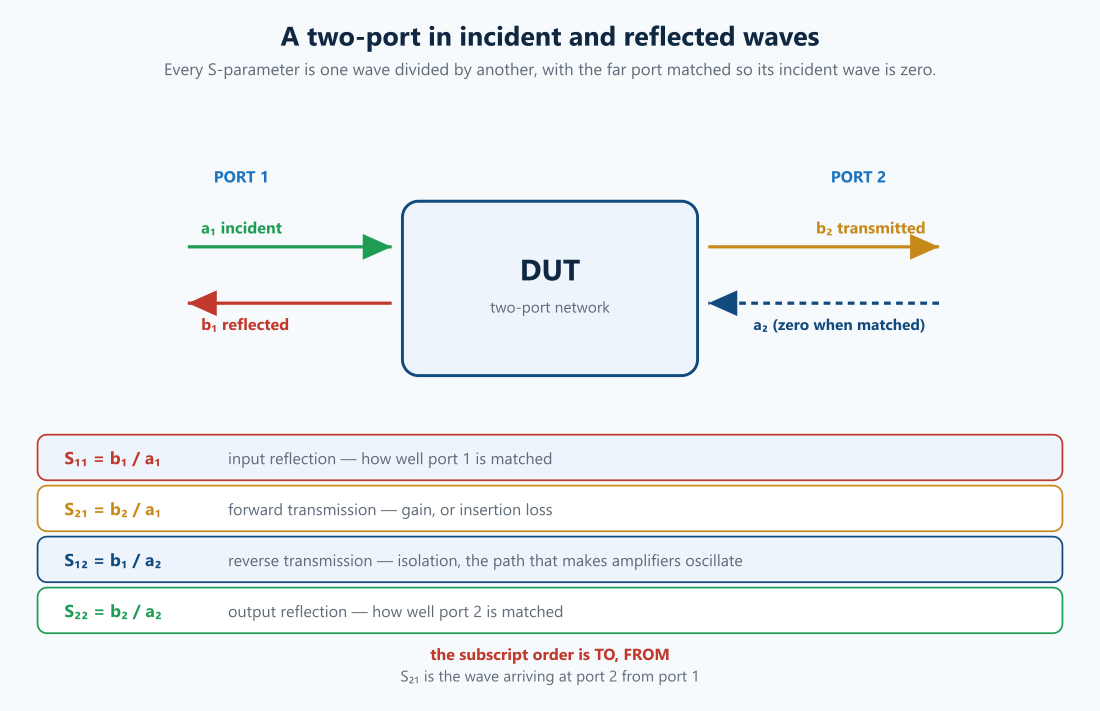
Every port has an incident wave going in and a reflected wave coming back, normalised so that their squared magnitudes are power:
For a two-port, written out:
Each parameter is defined with the other port matched, so its incident wave is zero:
| Parameter | Definition | Name | What it tells you |
|---|---|---|---|
| , with | input reflection | how well port 1 is matched | |
| , with | forward transmission | gain, or insertion loss | |
| , with | reverse transmission | isolation, and the feedback path that makes amplifiers oscillate | |
| , with | output reflection | how well port 2 is matched |
The subscript order is “to, from”, not “from, to”. is the wave arriving at port 2 from port 1. Getting this backwards is the single most common beginner error, and it is silent on a symmetric device — which is exactly where you will not notice it.
Reference impedance is part of the data
S-parameters are meaningless without the impedance they are referenced to, almost always 50 Ω, sometimes 75 Ω for video and cable, and occasionally per-port differing values. The same physical device has different S-parameters in a 50 Ω and a 75 Ω system. A Touchstone file states it on its option line; a datasheet plot sometimes does not, and then you have to ask.
3. Reflection, and everything derived from it
For a one-port, is the reflection coefficient:
Worked, in a 50 Ω system:
| Load | Angle | ||
|---|---|---|---|
| 50 Ω (matched) | 0 | 0.0000 | — |
| 75 Ω | +0.2000 | 0.2000 | 0° |
| 100 Ω | +0.3333 | 0.3333 | 0° |
| 25 Ω | −0.3333 | 0.3333 | 180° |
| Short (0 Ω) | −1 | 1.0000 | 180° |
| Open (∞) | +1 | 1.0000 | 0° |
| 50 + j50 Ω | 0.2 + j0.4 | 0.4472 | 63.4° |
Notice that a short and an open both reflect everything — they differ only in phase. That 180° difference is what makes them useful as calibration standards, and it is the whole reason the Smith chart is a polar plot.
From everything else follows:
| Return loss | VSWR | Power reflected | Mismatch loss | |
|---|---|---|---|---|
| 0.010 | 40.0 dB | 1.020 | 0.01% | 0.000 dB |
| 0.032 | 30.0 dB | 1.065 | 0.10% | 0.004 dB |
| 0.100 | 20.0 dB | 1.222 | 1.00% | 0.044 dB |
| 0.200 | 14.0 dB | 1.500 | 4.00% | 0.177 dB |
| 0.333 | 9.5 dB | 2.000 | 11.11% | 0.511 dB |
| 0.500 | 6.0 dB | 3.000 | 25.00% | 1.249 dB |
Return loss is quoted as a positive number by convention, and larger is better — 40 dB is an excellent match, 6 dB is a bad one. You will also see it written as a negative in dB, which means the same thing with the opposite sign. Both conventions are in daily use and the only defence is to look at whether the number gets bigger or smaller as the match improves.
Mismatch loss is the useful one and the least quoted. It is the power you fail to deliver because of reflection. Read the table: even a mediocre 14 dB return loss only costs you 0.18 dB of delivered power. That is why chasing return loss past a point is often wasted effort — the reflected energy matters far more for what it does elsewhere (re-reflections, resonances, crosstalk into neighbours) than for the power it removes.
4. Transmission
| Insertion loss | Power through | |
|---|---|---|
| 1.000 | 0 dB | 100% |
| 0.891 | 1 dB | 79.4% |
| 0.708 | 3 dB | 50.1% |
| 0.500 | 6 dB | 25.0% |
| 0.316 | 10 dB | 10.0% |
| 0.100 | 20 dB | 1.0% |
For an amplifier and the same quantity is gain. For anything passive it is loss, and always.
5. More than two ports
An -port has an matrix, so the data grows quadratically:
| Ports | File | Matrix | Complex numbers per frequency |
|---|---|---|---|
| 1 | .s1p | 1×1 | 1 |
| 2 | .s2p | 2×2 | 4 |
| 4 | .s4p | 4×4 | 16 |
| 12 | .s12p | 12×12 | 144 |
| 32 | .s32p | 32×32 | 1024 |
A 32-port file at 10,000 frequency points holds about 20 million numbers. This is why full-board extractions get unwieldy, and why port count is a design decision in itself.
Port numbering is the most expensive convention in the field
There is no universal standard for how ports on a differential structure are numbered. Two conventions dominate:
- 1-2 / 3-4 — port 1 and 2 are the two ends of the first single-ended line, 3 and 4 the second.
- 1-3 / 2-4 — ports 1 and 2 are the two lines at the near end, 3 and 4 at the far end.
Both are common. Both produce a valid-looking file. Feeding one into a tool expecting the other silently swaps a through-path for a crosstalk path, and the result looks like a badly designed structure rather than a mis-wired file. Always check the port map, and sanity-check by plotting: should look like a through path, not like a coupling curve.
Mixed-mode S-parameters
For a differential pair, single-ended parameters are not what you want. The four-port matrix is transformed into modal quantities:
- — differential in, differential out: the real insertion loss of the pair.
- — common-mode transmission.
- — mode conversion: differential in, common out. This is the one that causes EMC failures, and it is zero for a perfectly symmetric structure. It is never zero.
- — common in, differential out: how external common-mode noise gets into your signal.
The mode-conversion terms are the whole reason to look at mixed-mode data. A pair can have excellent and still radiate, and only shows it.
6. The Touchstone file
A plain-text format, originally from EEsof, now standardised as IEEE Std 370‘s companion and maintained as Touchstone 2.0 by the IBIS Open Forum.
! A 2-port file: comments start with an exclamation mark
# GHz S MA R 50
!freq      |S11|   /_S11   |S21|   /_S21   |S12|   /_S12   |S22|   /_S22
0.0        0.0100  0.00    0.9990  0.00    0.9990  0.00    0.0100  0.00
1.0        0.0316 -45.00   0.9487 -36.00   0.9487 -36.00   0.0316 -45.00
10.0       0.1000 -90.00   0.7080 -180.0   0.7080 -180.0   0.1000 -90.00
The option line
The line beginning # sets how every number is to be read:
| Field | Options | Meaning |
|---|---|---|
| Frequency unit | HzkHzMHzGHz | what the first column is in |
| Parameter | SYZHG | almost always S |
| Format | MADBRI | magnitude-angle, dB-angle, real-imaginary |
Rn | e.g. R 50 | the reference impedance |
All three formats describe the same number. One value, three spellings:
| Format | Written as | Meaning |
|---|---|---|
MA | 0.316228 -45.0000 | magnitude 0.3162, angle −45° |
DB | -10.000000 -45.0000 | −10 dB, angle −45° |
RI | 0.223607 -0.223607 | real and imaginary parts |
Angles are always in degrees, never radians — including in RI files, where there are no angles at all. And in DB format the magnitude is , not : these are wave amplitudes, not powers.
The two-port ordering trap
This is the one that costs real time. In Touchstone 1.0, a two-port file lists its four values in the order:
That is column-major — comes second. But for three ports and above, the data is row-major: , then , and so on.
So the two-port case is the exception, and a parser written for the general case gets and backwards on every two-port file it reads. On a reciprocal passive structure and nothing appears wrong — until the file describes an amplifier or an isolator, where the two differ by 30 dB and the error is enormous. Touchstone 2.0 fixes this with an explicit [Two-Port Data Order] keyword; 1.0 files remain overwhelmingly common.
Other things that bite
- No blank-line or ordering guarantees. Frequencies should ascend; not all writers comply.
- Noise data may follow the S-parameter block in a two-port file, with a different column layout entirely. A naive parser reads it as more S-data.
- Version 2.0 adds
[Version],[Number of Ports],[Reference]for per-port impedances, and[Network Data]— worth preferring when a tool will write it. - Frequency spacing sets the time-domain window if you convert to an impulse or step response. The window is and the resolution is :
| Spacing | Points | Span | Time window | Resolution |
|---|---|---|---|---|
| 50 MHz | 200 | 10 GHz | 20 ns | 100 ps |
| 10 MHz | 1000 | 10 GHz | 100 ns | 100 ps |
| 1 MHz | 10000 | 10 GHz | 1000 ns | 100 ps |
Too coarse a spacing wraps the impulse response around the window, and the wrapped energy looks exactly like a reflection that is not there.
7. The checks every file should pass
Run these on everything, including vendor models. Especially vendor models.
Passivity. A passive structure cannot emit more energy than it absorbs. For a two-port, at every frequency:
| Case | Verdict | |
|---|---|---|
| Ideal thru | 1.000 | lossless, the boundary |
| Good match, low loss | 0.9998 | passive |
| Lossy component | 0.500 | passive — half the energy absorbed |
| 1.153 | impossible |
The general form is that the eigenvalues of must be non-negative. Measured data violates this slightly almost always, from noise; large violations mean a broken model.
Reciprocity. For any passive structure without ferrites or active devices, . Violation means either a non-reciprocal device — or a mis-wired file.
Causality. The response cannot precede the stimulus. This shows up as a magnitude and phase that are not Hilbert-transform pairs, and its practical symptom is a time-domain step response that starts before time zero. Non-causal data usually means a missing DC point or a non-physical material model.
DC behaviour. Extrapolation to 0 Hz must be physical. Many tools need a real DC point and will invent one badly if it is absent.
A monotonic-ish insertion loss with no unexplained nulls. A null means a resonator — a via stub, a cavity, a bad termination — and it is either real and important, or an artefact.
8. What you actually do with them
- Cascade. Convert to T-parameters, multiply, convert back — that is how a die, package, connector, cable and board become one channel. The reference planes must match at every junction, and mismatched planes are the most common cascading error.
- Simulate. Convolve with a driver and receiver model to get a time-domain eye.
- De-embed. Remove a fixture’s contribution to see the device alone — TRL, or 2x-thru per IEEE 370.
- Design. Amplifier gain, stability and noise all come straight from the S-matrix, as in part three of the series.
- Correlate. Overlay measured against simulated. A model you have never compared to a measurement is a hypothesis.
Where we fit
We characterise and model the passive structures that these files describe — connectors, launches, via transitions, cables and board channels — in Ansys HFSS and SIwave, and correlate them against VNA measurements. When a vendor’s file does not match the bench, working out which one is wrong is a large part of the job.
If you have a Touchstone file you do not trust, or a channel that will not close, that is the conversation we like having.
Glossary
a, b waves — Normalised incident and reflected travelling waves, defined so that and are powers in watts. Everything else here is a ratio of these. The normalisation is why S-parameters compose cleanly through a cascade while impedance parameters do not.
Causality — The response cannot precede the stimulus. It sounds like philosophy and is a practical data check: causal data satisfies the Kramers–Kronig relations linking magnitude and phase, and a file that violates them produces a time-domain step that starts moving before the edge arrives. Simulators either refuse such a file or quietly “fix” it, and the fix changes your answer.
De-embedding — Removing a fixture’s contribution so the numbers describe the device rather than the launch, the connector and the trace that got you there. At multi-gigahertz the fixture is often worse than the DUT, so the de-embedding is not a refinement — it is the measurement. Common methods: TRL, 2x-thru (AFR/IEEE 370), and port extension for phase only.
Insertion loss — ; how much fails to get through. Note it lumps together what was absorbed and what was reflected, which is why a filter’s stopband shows enormous insertion loss while dissipating almost nothing — it is sending the energy back, not eating it.
Mismatch loss — The portion of insertion loss caused purely by reflection, . Worth separating from dissipative loss because they behave differently in a cascade: dissipated power is gone, reflected power re-reflects and produces ripple. VSWR 2:1 is only 0.51 dB of mismatch loss, which is why chasing return loss past about 15 dB rarely pays.
Mixed-mode S-parameters — The differential/common-mode recasting of a four-port into four 2×2 blocks: (differential through and reflected), (common-mode), and the cross blocks and . A differential pair’s real behaviour lives in and ; the single-ended four-port describes the same device in a basis nobody designs in.
Mode conversion () — Differential energy becoming common-mode through asymmetry — unequal trace lengths, a via on one side only, a connector pin-out that breaks symmetry. Common-mode current radiates where differential does not, so this is the usual root cause of a differential pair failing EMC, and it is invisible in a plot that looks fine.
Passivity — A passive network cannot emit more energy than it absorbs; formally, the singular values of the S-matrix are all at every frequency. A passivity violation in a model is an extrapolation artefact or a bad fit, and it makes a transient simulation grow without bound — the classic “my SerDes sim exploded” cause.
Reciprocity — . True of any network built from ordinary materials, and deliberately broken by magnetically biased ferrites — which is the entire basis of the isolator and circulator. If a passive measurement comes back non-reciprocal, suspect the calibration before the physics.
Reference impedance — The system impedance the parameters are defined against, usually 50 Ω. It is part of the data, not a detail: the same device has different S-parameters at 50 Ω and at 100 Ω differential, and re-normalising between them is a real calculation. A Touchstone file that omits it, or whose header disagrees with the measurement, is silently wrong.
Return loss — , quoted as a positive number, where bigger is better. Often confused with its own negation: a datasheet showing “−15 dB return loss” means dB, which is 15 dB of return loss. Both conventions are in circulation; read the axis.
Touchstone — The .sNp text format S-parameters are exchanged in, where N is the port count. The header line carries the frequency unit, the parameter type, the format (dB/angle, magnitude/angle, real/imaginary) and the reference impedance. Version 2.0 adds a port-order and mixed-mode description that v1 files leave to a filename convention and hope.
VSWR — , the standing-wave ratio on the line. The same information as return loss in a scale that runs from 1 to infinity instead of infinity to zero. It survives because a VSWR meter measures it directly, and because power-handling and ruggedness specifications are written in it.
Further reading — reference books
Book links below are Amazon affiliate links: if you buy through one we earn a small commission at no extra cost to you. It does not influence what is recommended — the same books were on this list before the links were.
- David Pozar, Microwave Engineering — the standard derivation of scattering parameters.
- Joel Dunsmore, Handbook of Microwave Component Measurements — the best book on measuring them properly, and on what goes wrong.
- Eric Bogatin, Signal and Power Integrity — Simplified — the SI-side treatment.
- Stephen Hall & Howard Heck, Advanced Signal Integrity for High-Speed Digital Designs.
- IEEE Std 370-2020, on fixture de-embedding and the quality metrics that make a file auditable.
- The IBIS Open Forum’s Touchstone 2.0 specification.
Have a Touchstone file you do not trust, or a channel that will not close? That’s what we do. Reach us at circuit-design.space.
circuit-design.space · +1-971-357-1400 · anovickis@circuit-design.space