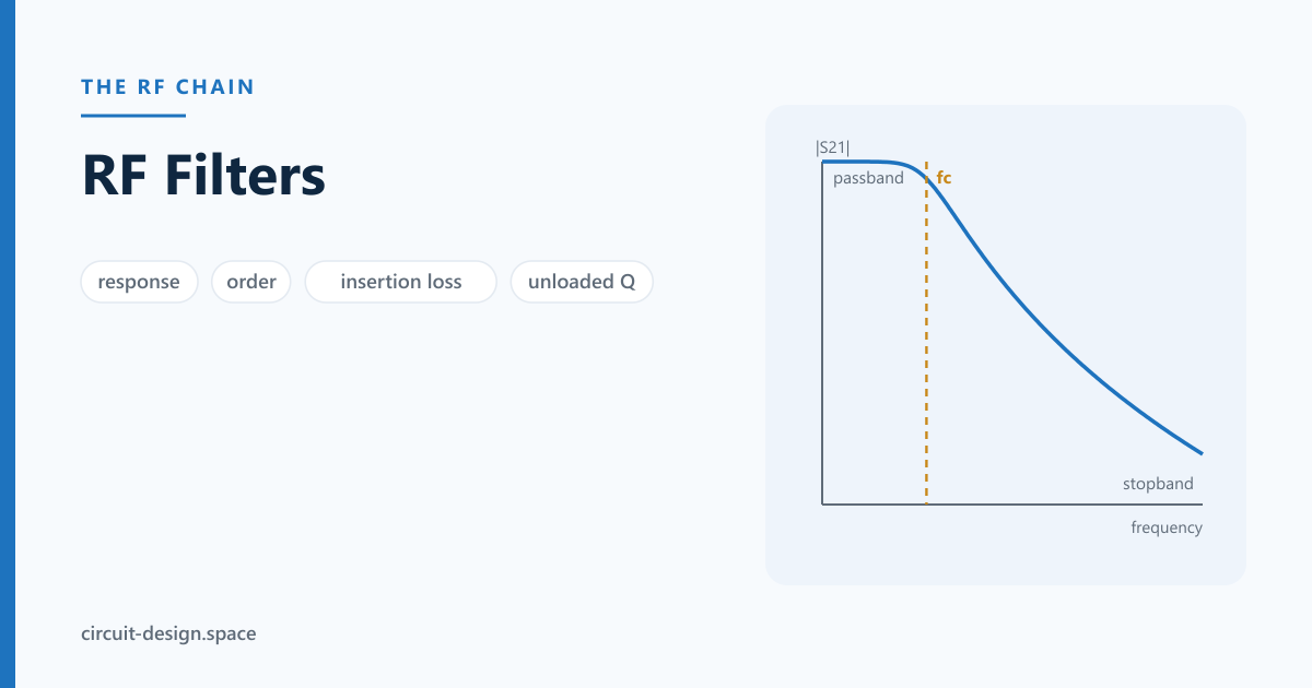
Part of the RF chain series — a page per block. The filter sits between the antenna and the LNA, which is the most consequential position it can occupy.
The RF chain, block by block —Antenna · Filter · LNA · Mixer · LO · IF & ADC · PA · Isolator · Coupler · Overview
A filter’s job is to pass one band and reject others. The difficulty is that every mechanism for rejecting out-of-band energy also costs something in band — insertion loss, group-delay distortion, size, or money — and in a receiver front end the thing it costs is noise figure.
1. The position problem, first
A filter in front of an LNA adds its insertion loss to the system noise figure, one for one. A 2 dB pre-select filter makes a 1.2 dB LNA into a 3.2 dB front end before anything else happens. That is the central tension in receiver design: you want selectivity early to stop big interferers reaching the LNA, and you want loss late so it does not cost noise.
The usual resolution is a shallow, low-loss pre-select filter in front and the sharp selectivity after the LNA’s gain, where a few dB of loss is nearly free by the Friis cascade. Getting this ordering wrong is the most expensive filter mistake available.
2. Responses
There is no best response, only a choice about where to spend the compromise:
| Response | Passband | Rolloff | Group delay | Use it when |
|---|---|---|---|---|
| Butterworth | maximally flat | gentle | moderate | you want flat amplitude and can afford order |
| Chebyshev | equiripple | steeper | worse | rejection matters more than flatness |
| Inverse Chebyshev | flat | steep | moderate | ripple is acceptable in the stopband, not the passband |
| Elliptic (Cauer) | equiripple | steepest | worst | you need maximum rejection in minimum order |
| Bessel | flat | poor | flat | pulses and modulation must not be distorted |
Bessel is the one people forget. Every other response trades group-delay flatness for rolloff, and group-delay variation smears a modulated signal — it shows up as EVM, not as amplitude error. For a wideband digitally modulated signal, a sharp elliptic filter can pass the amplitude mask perfectly and still ruin the constellation.
3. Order sets rejection, and the arithmetic is simple
For a Butterworth response:
| Order | at | at | at | at |
|---|---|---|---|---|
| 3 | 10.9 dB | 18.1 dB | 28.6 dB | 60.0 dB |
| 5 | 17.7 dB | 30.1 dB | 47.7 dB | 100.0 dB |
| 7 | 24.7 dB | 42.1 dB | 66.8 dB | 140.0 dB |
| 9 | 31.7 dB | 54.2 dB | 85.9 dB | 180.0 dB |
Read the first column. Close-in rejection is expensive: to get 30 dB at 1.5× the corner you need order 9 in Butterworth, where an elliptic response would do it in 5 at the cost of passband ripple and group delay. That column is why elliptic filters exist and why the image frequency’s distance from the signal — set by the IF choice — matters so much. A high IF puts the image far out the rejection curve where a cheap filter is adequate.
The same requirement, priced in each response
Butterworth is the expensive way to buy rejection. The order each response needs for a given stopband requirement, computed rather than asserted:
| Rejection at | Butterworth | Chebyshev 0.1 dB | Chebyshev 0.5 dB |
|---|---|---|---|
| 30 dB at 1.5× | 9 | 7 | 6 |
| 40 dB at 1.5× | 12 | 8 | 7 |
| 60 dB at 1.5× | 18 | 10 | 9 |
| 40 dB at 1.2× | 26 | 12 | 11 |
| 40 dB at 2.0× | 7 | 6 | 5 |
Three readings, all useful. Accepting 0.1 dB of passband ripple removes a third of the order — that is the cheapest trade on this page, and 0.1 dB of ripple is invisible to almost every system. Going from 0.1 dB to 0.5 dB of ripple buys almost nothing more — one order — so the standard advice to “use more ripple” has a floor. And the transition ratio dominates everything: 40 dB at 1.2× needs 26 Butterworth sections and 40 dB at 2.0× needs 7. If your filter is impossible, the frequency plan is what to change.
Where the order actually gets spent: insertion loss
Each order costs insertion loss, because each resonator has finite unloaded . The midband loss of a bandpass filter is close to:
where FBW is the fractional bandwidth and are the lowpass prototype element values. For Butterworth, , so is 2.83 at , 4.00 at , 6.47 at , 8.99 at .
The coefficient is , and it is worth seeing where it comes from rather than taking it on trust — it is the number most often misremembered as 4.343. A resonator with loaded in a structure of unloaded passes amplitude ; of them cascade, so ; and of that is . For the normalised prototype , which gives the form above.
For a third-order Butterworth bandpass (), midband insertion loss in dB:
| FBW | = 100 | 200 | 500 | 2000 | 5000 |
|---|---|---|---|---|---|
| 1% | 34.74 | 17.37 | 6.95 | 1.74 | 0.69 |
| 2% | 17.37 | 8.69 | 3.47 | 0.87 | 0.35 |
| 5% | 6.95 | 3.47 | 1.39 | 0.35 | 0.14 |
| 10% | 3.47 | 1.74 | 0.69 | 0.17 | 0.07 |
| 20% | 1.74 | 0.87 | 0.35 | 0.09 | 0.03 |
Sanity-check the far column against parts you can buy: a 2% three-pole cavity filter at 0.35 dB is exactly where real cavity filters are specified, which is the quickest way to confirm the arithmetic is the right arithmetic.
This single table decides most filter technology choices, and it does so before any layout exists. A 2% bandpass in microstrip () costs 8.7 dB — which, in front of an LNA, is 8.7 dB of noise figure and the design is not merely compromised, it is dead. The same filter in a cavity () costs 0.35 dB. That is not a refinement; it is the difference between a product and a rebuild.
The corollary is the rule of thumb worth carrying: loss scales as and linearly with , so halving the bandwidth doubles the loss, and going from 3rd to 7th order rather more than doubles it. Do this arithmetic on the back of an envelope before committing to a technology — it takes a minute and it is the single highest -value minute in filter selection.
Typical unloaded Q, to use with the table:
| Resonator | |
|---|---|
| Lumped LC, 0402 parts | 40–100 |
| Microstrip | 150–250 |
| Stripline | 200–400 |
| Ceramic / LTCC | 300–800 |
| BAW / FBAR | 1000–3000 |
| Dielectric resonator | 3000–10 000 |
| Air cavity | 3000–20 000 |
| SAW | ~10 000 (acoustic) |
4. Technologies
| Technology | Frequency | Q / selectivity | Insertion loss | Size | Notes |
|---|---|---|---|---|---|
| Lumped LC | < ~3 GHz | low–moderate | 0.5–3 dB | small | component Q limits everything |
| Microstrip / stripline | 1–40 GHz | moderate | 1–3 dB | area-hungry | free to fabricate, costs board space |
| Ceramic / LTCC | 0.5–10 GHz | good | 1–2 dB | very small | the volume-product default |
| SAW | 0.1–3 GHz | very high | 1–3 dB | tiny | sharp skirts, temperature drift, power-limited |
| BAW / FBAR | 1–6 GHz | very high | 1–2 dB | tiny | better than SAW above ~2 GHz, handles more power |
| Cavity / waveguide | > 1 GHz | extremely high | < 0.5 dB | large, heavy | base stations, radar, test equipment |
| Dielectric resonator | 1–40 GHz | very high | low | moderate | high-Q in less volume than cavity |
The pattern: Q buys selectivity and low loss, and you pay for Q in size. A cavity filter achieves what it does because it stores energy in air in a large volume. A SAW filter cheats by using acoustic waves — five orders of magnitude slower than electromagnetic ones, so a wavelength is microns rather than centimetres — which is why a phone can have a dozen of them.
SAW and BAW have two limits worth knowing: power handling (they are mechanical devices and can be damaged by a large transmit signal) and temperature drift (SAW more than BAW), which is why temperature-compensated variants exist.
5. From prototype to layout
The design flow that every filter textbook describes, compressed, because knowing the shape of it tells you where a design will fail.
Start from the normalised lowpass prototype. A table (or the formula above) gives element values for a 1 Ω source and a 1 rad/s corner. Everything after that is scaling.
Scale impedance and frequency:
Transform to bandpass. Each prototype inductor becomes a series LC, each capacitor a shunt LC, and the fractional bandwidth appears in the denominator:
And this is where narrowband designs die. As FBW shrinks, the series inductors grow and the series capacitors shrink — a 1% bandpass at 2 GHz asks for capacitors in the tens of femtofarads, which is smaller than the parasitic capacitance of the pad you would mount them on. The distributed equivalent is the same problem wearing different clothes: narrow bandwidth means weak coupling between resonators, which means coupling gaps too small to etch repeatably. A 0.05 mm gap that your fabricator holds to ±0.025 mm is a filter whose bandwidth is a lottery.
Three ways out, in ascending order of cost: widen the bandwidth if the system will tolerate it; move to a higher-, higher- technology where the same electrical gap is a larger physical one (ceramic, LTCC); or buy the filter as an acoustic or cavity part built by someone whose process is tuned for it. The third is usually right, and recognising it early saves a spin.
Then field-solve. At the point where coupling is set by a gap dimension, the closed-form synthesis has told you the topology and roughly the dimensions, and only a full-wave solve will tell you the answer — including the launches, the enclosure above the board, and the via fences beside it, all of which load the resonators.
6. Beyond the amplitude response
Group delay is the derivative of phase:
Flat amplitude with non-flat group delay distorts modulation; it is worst at the band edges of a sharp filter, which is exactly where a channel sits when the filter was designed to the channel width. Two quantitative hooks worth carrying:
- Group delay at band centre scales as — the same combination that set the insertion loss. A sharper, narrower filter is a slower filter, and in a TDD system that delay is part of the turnaround budget.
- Peak-to-peak group-delay variation across the channel is the number to specify, not the absolute delay. A flat 20 ns delays everything equally and does nothing; 20 ns of variation across a 20 MHz channel is a serious EVM contributor.
If a design needs both sharp rejection and flat delay, the answer is usually equalisation — an all-pass section, or a digital equaliser in the modem — rather than a different filter response. Bessel gives flat delay and almost no rejection; you generally cannot have both from the same passive network.
Return loss matters as much as insertion loss in a chain. A filter that rejects by reflecting — which all of them do — sends that energy back toward whatever precedes it. In front of a PA that is a ruggedness problem; between two stages it is a source of ripple as the reflections re-reflect.
Power handling and passive intermodulation. At transmit power levels, a filter’s own nonlinearity generates PIM. Ferrous metals, dissimilar-metal junctions and poor mechanical contacts in connectors are the usual culprits, and PIM lands in the receive band on a duplexed system.
Temperature. Ceramic and cavity filters drift with temperature; over an automotive or outdoor range the drift can be a significant fraction of the passband.
7. A selection method
- Write the mask: passband edges and ripple, stopband edges and required rejection, maximum insertion loss, group-delay limit.
- Find the hardest transition — the closest stopband edge relative to the passband — and compute the order that response type needs. If the order is absurd, the frequency plan is wrong, not the filter.
- Check what the insertion loss costs in its position: noise figure if before the LNA, output power and efficiency if after the PA.
- Check group delay against the modulation bandwidth.
- Choose the technology from Q, size and power handling.
- Field-solve any distributed structure. A microstrip filter is a coupled-resonator EM problem, and at its dimensions the pads and vias are part of it — see which solver to use.
- Measure over temperature and at power, not just at room temperature and small signal.
8. Example parts
For anything but a genuinely custom mask, buying beats building — the loss table in §3 is why. Illustrative parts; check current availability and the current datasheet.
LTCC lowpass, highpass and bandpass — the default for board-level filtering below ~10 GHz. Small, cheap, reasonable Q, and specified over temperature:
| Part family | What it is | Where it fits |
|---|---|---|
| Mini-Circuits LFCN series | LTCC lowpass, DC to a named corner | harmonic filtering after a PA, anti-alias ahead of an ADC |
| Mini-Circuits HFCN series | LTCC highpass | rejecting a low-frequency blocker or a strong LO leak |
| Mini-Circuits BFCN series | LTCC bandpass | pre-select in front of a wideband receiver |
| Johanson 2450BP15A100 | 2.45 GHz ceramic bandpass | the standard part in front of a 2.4 GHz radio |
| Murata LFB series | monolithic ceramic bandpass | volume ISM-band products |
Acoustic (SAW / BAW) — where the mask is steep and the band is standardised:
| Part family | Notes |
|---|---|
| Qorvo SAW filters | very sharp skirts below ~2 GHz; watch power handling and temperature drift |
| Qorvo / Broadcom BAW | better than SAW above ~2 GHz, more power, less drift |
| Murata SAW filters | wide catalogue of standardised cellular and ISM bands |
Common-mode chokes and EMI filters deserve a mention because they solve a problem that looks like a filter problem and is not: conducted emissions and common-mode currents on cables are a mode issue, not a frequency one, and a differential bandpass does nothing about them.
A useful shortcut when specifying: most catalogue filters are characterised into 50 Ω at both ports, and your circuit is not 50 Ω. Either match to it, or use the S-parameters the manufacturer publishes and simulate it in situ — a ceramic bandpass terminated in the actual input impedance of the LNA behind it can look nothing like its datasheet plot. Download the Touchstone file and check; most vendors now publish them.
9. The pitfalls
- A sharp filter in front of the LNA — selectivity bought with noise figure.
- Choosing the technology before doing the loss arithmetic.
- A narrowband printed filter whose coupling gaps are below the fabricator’s tolerance.
- Reading a catalogue filter’s plot without checking it is terminated the way your board terminates it.
- Designing to the amplitude mask and ignoring group delay, then failing EVM.
- Assuming a lumped design works at a frequency where its components have self-resonated: every capacitor is an inductor above its SRF; see power integrity for the same effect.
- Simulating a microstrip filter with ideal line models rather than a field solver.
- Ignoring PIM on a duplexed system.
- SAW filters in a transmit path that exceeds their power rating.
- Forgetting that a filter’s rejected energy is reflected, and lands somewhere.
Further reading
- Jia-Sheng Hong, Microstrip Filters for RF/Microwave Applications. The modern standard; the insertion-loss and coupled-resonator results above are its bread and butter.
- Randall Rhea, HF Filter Design and Computer Simulation. Practical, and honest about what happens between the synthesis and the board.
- Matthaei, Young and Jones, Microwave Filters, Impedance-Matching Networks, and Coupling Structures. The 1964 classic. Still the source everyone else is citing.
- Anatol Zverev, Handbook of Filter Synthesis. The tables, if you ever need to do it without a computer.
- David Pozar, Microwave Engineering. Chapter 8 is the cleanest short introduction to the prototype-and-transform method.
The RF chain, block by block —Antenna · Filter · LNA · Mixer · LO · IF & ADC · PA · Isolator · Coupler · Overview
Glossary
Bessel — The response with maximally flat group delay and poor rolloff. The one people forget, and the right choice when a modulated signal must not be smeared — a sharp elliptic filter can pass the amplitude mask perfectly and still ruin the constellation.
Butterworth / Chebyshev / elliptic — Maximally flat, equiripple, and equiripple-in-both-bands respectively, in increasing order of rolloff and decreasing order of passband manners. Accepting 0.1 dB of ripple removes about a third of the order, which is the cheapest trade available; going from 0.1 to 0.5 dB buys almost nothing more.
Coupling coefficient — How strongly adjacent resonators are coupled, set by a gap dimension in a printed filter. Narrow bandwidth means weak coupling means small gaps — and a 0.05 mm gap held to ±0.025 mm is a filter whose bandwidth is a lottery.
Fractional bandwidth (FBW) — Bandwidth divided by centre frequency. It appears in the denominator of both the insertion loss and the group delay, so halving it doubles both. The single most consequential number in a filter specification.
Group delay — . What matters is the peak-to-peak variation across the channel, not the absolute value: a flat 20 ns delays everything equally and does nothing, while 20 ns of variation across 20 MHz is a serious EVM contributor.
Order — The number of poles, and what buys rejection. Close-in rejection is expensive: 40 dB at 1.5× the corner needs order 12 in Butterworth and 8 in Chebyshev. If the order is absurd, the frequency plan is wrong rather than the filter.
PIM — Passive intermodulation: distortion generated by a passive structure at high power, from ferrous metals, dissimilar-metal junctions and poor mechanical contacts. Lands in the receive band on a duplexed system, and it is a mechanical problem as much as an electrical one.
Prototype g-values — The normalised element values a filter is synthesised from, for a 1 Ω source and a 1 rad/s corner. Everything after that is impedance and frequency scaling, and is what the insertion-loss formula needs.
Ripple — Passband amplitude variation, traded for rolloff. It is specified in dB and it is cheap: 0.1 dB is invisible to almost every system and removes a third of the order.
SAW / BAW — Acoustic filters. They cheat by using waves five orders of magnitude slower than electromagnetic ones, so a wavelength is microns and a phone can hold a dozen. Two limits worth knowing: power handling, because they are mechanical, and temperature drift — SAW more than BAW.
Transition ratio — The stopband edge divided by the passband edge. It dominates everything: 40 dB at 1.2× needs 26 Butterworth sections and at 2.0× needs 7. When a filter looks impossible, this is the number to change.
Unloaded Q () — The resonator’s own quality factor, and what buys low loss. Midband loss goes as , so and fractional bandwidth together decide the technology before any layout exists. You pay for in size: a cavity filter works because it stores energy in air, in volume.
Related
- The RF chain overview
- The antenna in front
- The LNA behind — where filter loss becomes noise figure
- The mixer — image rejection is a filter problem set by the IF
- Smith chart — matching the filter’s ports
Have a filter mask that will not close, or a front end where selectivity is costing too much noise? That’s what we do. Reach us at circuit-design.space.
circuit-design.space · +1-971-357-1400 · anovickis@circuit-design.space